The basic idea
The basic idea we have for reading the time (or any other analog device!) is to first capture an image of the device using a web camera and use the image processing tools in Sympathy for Data to read the hour and minute hands from the clock. Our goal is to do this with only the open-source image processing tools that are included in Sympathy for Data, and no custom code.
Our aim is not to create a solution that works for any image of any clock, but rather to show how we can reliably read the values of the given clock given a very specific camera angle and lighting situation. To do this for any clock and lighting setup requires more advanced techniques, often involving machine learning, and which harder to guarantee that it works in all of the target situations.
For the purpose of this blog post, we will not be using machine learning or any other advanced algorithms but rather rely on basic (traditional) image processing techniques. This problem resembles very much that of designing image processing algorithms that are used every day in industrial production — where you have a highly controlled environment and want simple and fast algorithms. By controlling the environment we can make this otherwise complex task very simple and easy to design an algorithm for. When doing image processing for industrial purposes it is commonly found that you can simplify the problem and increase robustness by heavily controlling the environment and the situation in which your images are acquired.
For the impatient, you can download the dataset with images that we prepare in the first part as well as the finished Sympathy for Data workflow.
Acquiring the data
Step one is to acquire some images of the clock and to try to analyse them in Sympathy. If you don’t want to repeat these steps yourself you can simply download the full dataset from here.
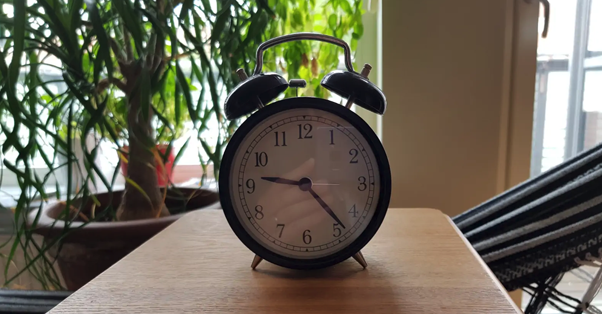
We start with a naive approach and just place the web camera in front of the clock and record images once per minute over a full day. Some example of these images are below:
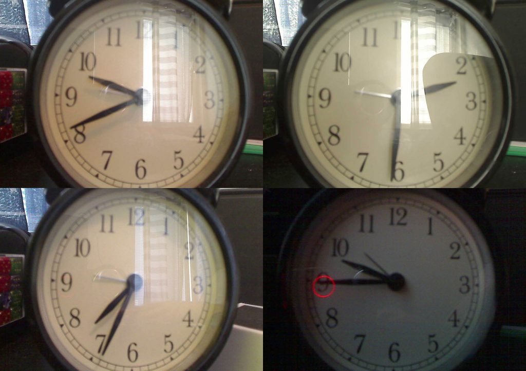
What we can see in the images above is two main problems: the lighting varies widely depending on the time of day, and the lighting in the image itself varies widely due to specular reflections and makes part of the hour-hand invisible second image above. Whatever algorithm we come up with will have a hard time to deal with an invisible hour-hand.
We can also note that with a stronger and directional light we would have shadows cast by the hour and minute arms of the clock is projected at different part of the face of the clock depending on the incoming light direction. If we where to directly try to analyse these images we would need to compensate for the shifting position of the shadows, and we could not use any simple thresholding steps since the overall light changes widely. Any algorithms we create for these kind of images will inherently be more complex and possibly more prone to failures when the light conditions change. We would need to test if over a wide range of conditions (day, night, sunset, rainy weather, sunny weather, summer, winter) to be sure that it works correctly under all conditions.
An attempted first fix for the specular reflections was to remove the cover-glass of the clock, the idea being that the face paint of the clock wouldn’t be reflective enough to give these issues. This however wasn’t enough to solve the problem with disappearing arms for all lighting conditions, and are we to apply this idea to an industrial setting it may oftentimes not be possible to make such a modification. A better solution is therefore to remove all direct light in favour of a setup with only diffuse lights.
To solve both these problems we choose to make a controlled environment with only diffuse light and where we know that the only thing that changes are the positions of the clock’s arms. We force a constant light level by enclosing the clock and camera in a box with a lightsource. This way we can also eliminate the the shadows of the clocks arms by placing the lightsource from the same direction as the camera.
Building a camera friendly light source
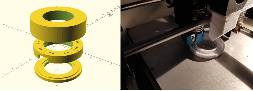
In order to eliminate the shadows from the clock arms and to provide a even and diffuse lighting conditions we place a ring of white LED’s around the camera. Usually this is done using professional solutions such a light ring for photography, but we’ll manage with a simple 3d-printed design and some hobby electronics. You can find the downloads for these over a Thingiverse.
The design for this light is simple ring where we can add the lights plus a diffuser on top of it to avoid any sharp reflections.
After printing the parts above we place a number of white LED’s in the small holes in the middle part above. By twisting the pins together with each other on the underside (take care with the orientation of anode and cathode!) we can easily keep them in place while at the same time connecting it all up. See if you can spot the mistake I did below in the wiring. Fortunately it was salvageable.
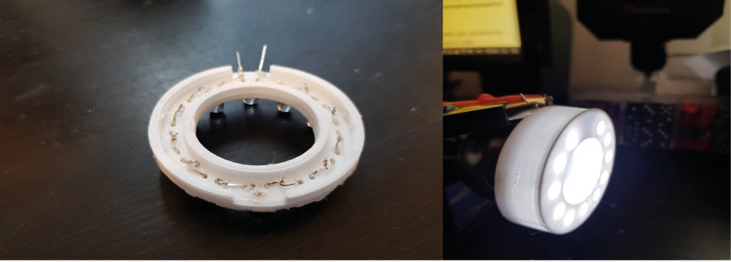
Next step is to place the diffuser over the LED’s and to attach it onto your web camera. Power it with approximately 3V per LED used. Point it straight at the clock and put an enclosure over it. We can used a simple carton box as a simple enclosure that removes all external light.
Congratulations, you can now get images of the clock with perfect lighting conditions regardless of sunlight, people walking bye, or any other factors that would complicate the readings.
Pre-processing the images
When doing image processing it is common to operate on grayscale images unless the colour information is an important part of the recognition task. For this purpose we first run a pre-processing step on the whole dataset where we convert the images to greyscale and downsample since we don’t need the full resolution of the camera for the rest of the calculations. This can easily be done using Sympathy for Data.
First create a new flow and point a Datasources directory to a copy of the dataset (we will overwrite the files in place). Add a lambda node by right clicking anywhere in the flow and select it. Connect a map node to apply the lambda for every datasource found.
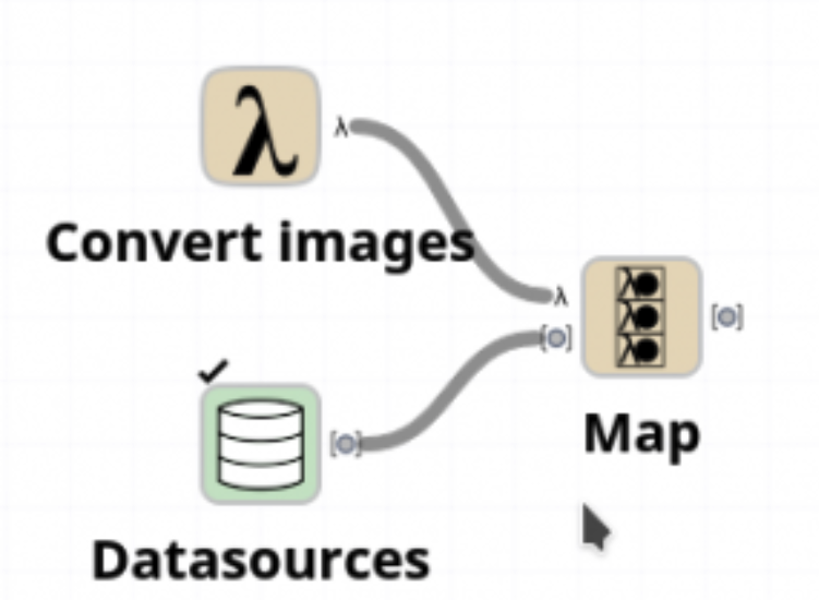
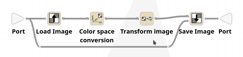
Before you can run it, add the nodes below into the lambda node to do the actual image conversion. You need to select greyscale in the configuration menu of the colour space conversion node, and rescale X/Y by 0.5 in the transform image node. Note that the “save image” node here overwrites the images in place, so try not to run the node until everything is ok. Another option would be to compute a new filename to be used instead using eg. a datasource to tables node and a calculator node.
In the dataset that you can download we have already done these conversions (downscaling to 800×500 pixels) to save on bandwidth.
Analysing the images
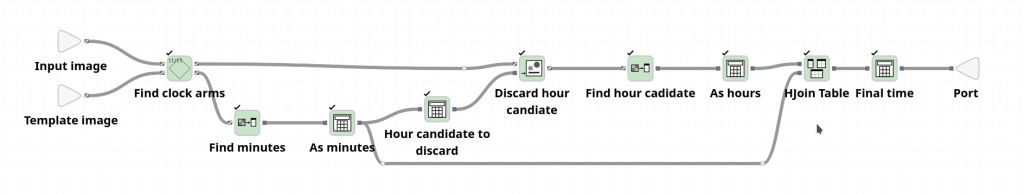
Our goal in this section is to create a Sympathy workflow that allows us to take any image of the clock and convert it into an hour and minute representation of the time.
Creating a template
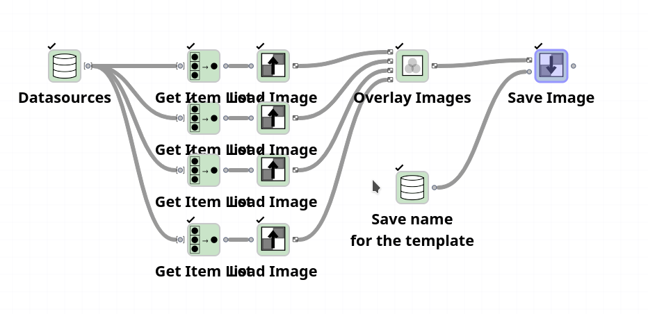
For the first step we want to extract only the arms of the clock that should be analysed. For this purpose we will use a practical trick to easily detect only the moving parts of the image. We do this by first calculating a template image that show how the images would look if all the moving parts were removed. This trick only works when the camera is fixed and there are no major changes in overall lighting.
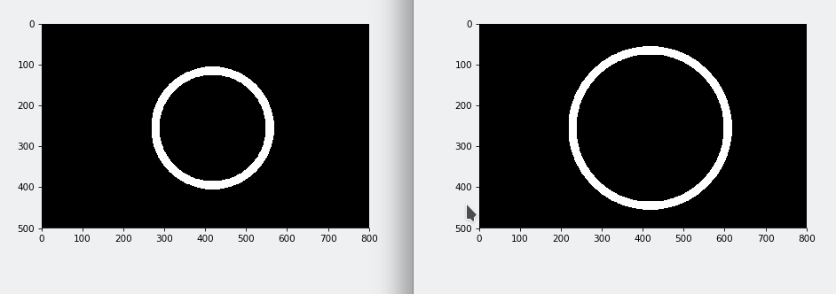
Start by calculating the median (or in our case max since we know the arm’s are black) of a few different images from the dataset. This will give an image where the arms of the clock is removed.
Select max as operator in the Overlay Images node below. This works since we know that the arms are darker than the background, and whichever pixel has a light colour in any of the images will have a light colour in the final image.
The results look surprisingly good given that we only used a few images (where the arms where all in different positions):

We save this template in a separate file so that we don’t have to redo the calculation for each image that should be processed.
Extracting the minute and hour arms
Continue by creating a new workflow and load one of the images to be analysed. We start by making a subtraction of the image to be analysed from the template image.
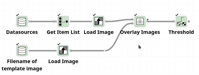
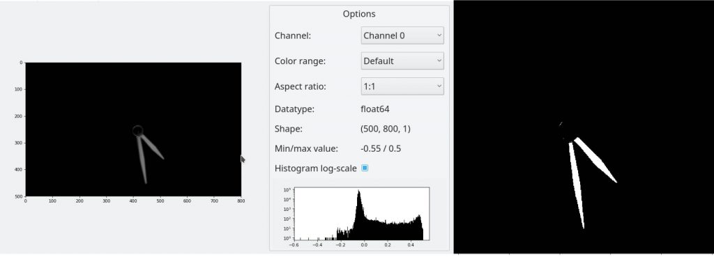
This will give an image where only the arms are visible, you will need to select “subtract” as the operation for the “overlay images” node.
The next step will be to perform a threshold to pick out only the arms of the clock as a binary image. To do so we use a Threshold node and set it to basic threshold. We can figure out a good threshold level by looking at the histogram above of the image after subtraction. We see that the maximum value of the image is 0.55 and that something significant seem to happen around the 0.4 mark (note that the graph is logarithmic!). We set the threshold to 0.35 and get the results shown above.
Since there can be some small smudges and missed spots on the binary image we apply morphological closing on the image using a structuring element of size 20 which should be more than enough to compensate for any missed pixels caused by noise, scratches on the object/lens or the otherwise black areas of the image.

Finally, we can note that we only actually need to see the tips of the hour and minute hand in order to read the time. If we sample to check for the the minute arm at every point in a circle with a radius closer to the edge of the picture we can know which pixels belong to the minute arm. Similarly, if we sample every point in in a smaller circle we get one or two sets of pixels corresponding to the hour arm when it is below the minute arm or both the hour arm and minute arm when they are not overlapping.
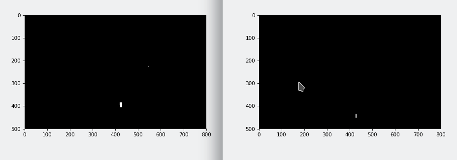
We can do this sampling by first creating two new templates that we use to select a subset of the pixels. This is done by drawing a white ring on an otherwise empty image for each of the two selections. We can do this using the Draw on image node and a Manually create table node that gives the XY coordinates (416, 256) and radius 200 for a circle with colour 1.0 and 170 for a circle with colour 0.0 — corresponding to the ring selecting the minute arm below:
After multiplying these two templates with the thresholded image (using again the overlay images node) we get two new images with blobs corresponding to the tips of the hour and minute hand:
All that is left now is to extract the coordinates of these blobs and to apply some math to convert them into hours and minutes.
Computing the minute
We can compute the position of the minute hand by using a Image statistics node with the algorithm “blob, DoG” with a threshold of 0.1. This algorithm finds “blobs”, or light area on a dark background, in an image by subtracting two low-pass (gaussian) filtered version of the image filtered at different scales.
All other parameters can be default, but the default value for threshold of the difference-of-gaussian algorithm is too high for our inputs.
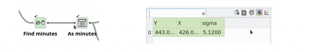
Now all we have to do is to convert the XY values 443, 426 of the tip of the minute hand into an actual value in the range 0 – 60. We can do this by calculating the vector from the center of the clock determined from the raw image as (416, 256) to the point of the detected blob. This gives us a vector (187, 10). By taking the arctan of this vector in a calculator node we can get the angle to this point and convert it into minutes. Note that we invert the y-component of this vector to compensate for the difference in coordinate systems (y-axis in images point down):
Computing the hours
In order to compute the hour we need to eliminate one of two possible candidates for the hour. Consider the blobs shown below, from just this data it is hard to know which hour it is:
However, what we can do is to take the position of the minutes that we calculate above and clear out one of the two blobs above. Since we know the radius that we used for the circle multiplied with the data, we can easily draw a black area on top of the location where the minute arm is located and at the given distance from the centre:
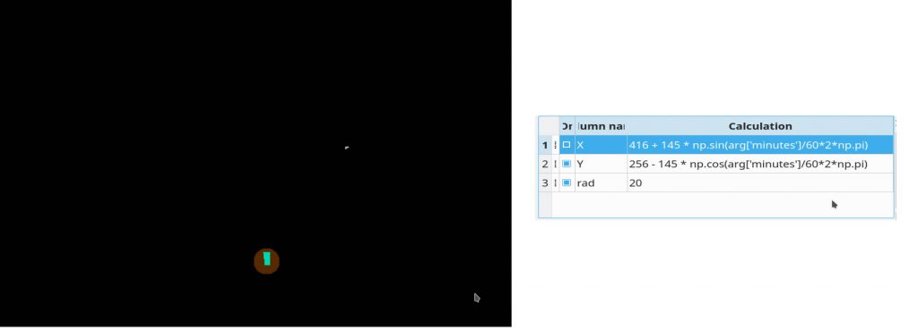
For this purpose we use another calculator node to compute the X/Y coordinate above and to draw a black circle onto the image at that location. For clarity it has been drawn as a brown circle in the example above to see what area of the image is deleted.
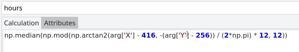
We extract the hour value from the remaining blob, if there is one, similarly as to how the minute value was calculated. Note that if there is no blob in the image containing the tip of the hour arm then the expression belows gives a NaN value. This happens when it is under the minute arm.
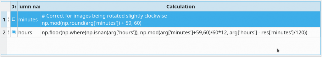
Finally, we can finish the flow by adding in a special case calculation that checks if the ‘hour’ column has the NaN value and if so instead derive the hour position from the minute position. In this step we also round the minutes to even number and round the hours down to nearest smaller integer. Note that we subtract a fraction of the minutes from the hours before rounding due to how the hour arm moves closer and closer to the next hour as the minutes raise.
We also subtract 1 (modulo 60) from the minute position since the captured images where all slightly rotated clockwise. We could have compensated this in the original pre-processing if we had noticed it earlier.
Time to check the results
Before we are happy with the flow, let’s check how well it performs versus the ground truth. Since the timestamp was saved when each image was captured we can easily compare these values with the results of the flow. Due to the sampling process and since the seconds of this clock wasn’t synchronized with the seconds of the computer sampling them — we should expect to be off by one minute in some of the readings.
As we can see in the table below we successfully read the time, with a difference of at most one minute, for first 100 images.
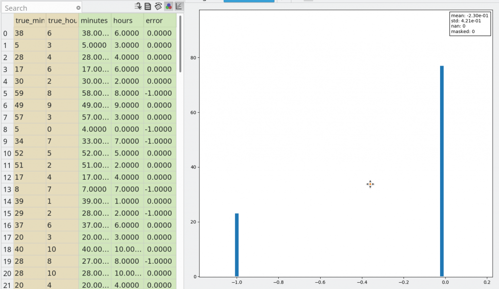
By only allowing ourselves to use the first 50 images when we developed the flow, and then validating it by running on a larger dataset we gain confidence that the algorithm works for all the situations it will encounter. We have run it the full dataset of 700+ hours without any other errors.

